Training Deep Neural Networks with Batch Normalization
Since its inception in 2015 by Ioffe and Szegedy, Batch Normalization has gained popularity among Deep Learning practitioners as a technique to achieve faster convergence by reducing the internal covariate shift and to some extent regularizing the network. We discuss the salient features of the paper followed by calculation of derivatives for backpropagation through the Batch Normalization layer. Lastly, we explain an efficient implementation of backpropagation using Python and Numpy.
Table of Contents:
- Background
- Forward Propagation through Batch Normalization layer
- Backpropagation through Batch Normalization layer
- Batch Normalization during test time
- Python Numpy Implementation
- How Powerful is Batch Normalization?
- Summary
Background
In 1998, Yan LeCun in his famous paper Effiecient BackProp highlighted the importance of normalizing the inputs. Preprocessing of the inputs using normalization is a standard machine learning procedure and is known to help in faster convergence. Normalization is done to achieve the following objectives:
- The average of each input variable (or feature) over the training set is close to zero (Mean subtraction).
- covariances of the features are same (Scaling).
- the correlation among features is minimum (Whitening).
The first two are easy to implement:
# Assume input data matrix X of size [N x D]
X -= np.mean(X, axis=0) # Mean subtraction
X /= np.std(X, axis=0)  # Scaling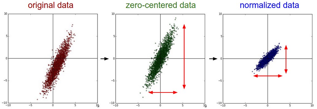
The third one requires decorrelating the features. However, the first two are sufficient to speed up the convergence, even when the features are not decorrelated. Moreover, whitening is note required for Convolutional Networks. For a detailed discussion on preprocessing, follow this link.
Why is normalization important ?
During backpropagation, we calculate \(\frac{\partial L}{\partial W} = x\frac{\partial L}{\partial y}\). Suppose the inputs to a particular neuron are all positive. The neuron will calculate the gradients of the loss with respect to weights associated with it (\(\frac{\partial L}{\partial w}\)) using this equation. Since all the components of \(x\) are positive, the gradients with respect to the weights are either all positive or all negative (depending upon the sign of \(\frac{\partial L}{\partial y}\)). Thus during stochastic gradient descent, \(W(t) = W(t-1) - \eta\frac{\partial L}{\partial W}\), the weights can only all decrease or all increase together for the given input pattern. This constrains the network to update weights by changing direction only through a zig-zag pattern, which is inefficient and slow. That is why we need to shift the input distribution towards zero mean (Mean subtraction) so as to increase the flexibility of the network. Also, scaling is necessary as it makes the weight contour less elliptical thereby directing the weights to converge in the right direction. You can play with this demo to convince how scaling helps in optimization.
The curse of internal covariate shift
As the inputs flow through the network, their distributions deviate from unit gaussian. In fact the input distribution at a particular layer depends on the parameters of all the preceding layers. The extent of deviation increases as the the network becomes deeper. Thus, merely normalizing the inputs to the network does not solve the problem. We need a mechanism which normalizes the inputs of every single layer. We can apply the same reasoning as we did earlier to prove that normalization of layer inputs helps in faster convergence.
We define Internal Covariate Shift as the change in the distribution of network activations due to the change in network parameters during training. Internal covariate shift is one of the reasons why training a deep neural network is so difficult.
- It requires careful hyperparameter tuning, especially learning rate and initial values of parameters.
- As the depth of the network increases, internal covariate shift becomes more prominent.
- The vanishing gradient problem is also linked with internal covariate shift.
Batch normalization to the rescue
As the name suggests, Batch Normalization attempts to normalize a batch of inputs before they are fed to a non-linear activation unit (like ReLU, sigmoid, etc). The idea is to feed a normalized input to an activation function so as to prevent it from entering into the saturated regime. Consider a batch of inputs to some activation layer. To make each dimension unit gaussian, we apply:
\[\hat{x}^{(k)} = \frac{x^{(k)} - E\big[x^{(k)}\big]}{\sqrt{\text{Var}\big[x^{(k)}\big]}}\]where \(E\big[x^{(k)}\big]\) and \(\text{Var}\big[x^{(k)}\big]\) are respectively the mean and variance of \(k\)-th feature over a batch. Then we transform \(\hat{x}^{(k)}\) as:
\[y^{(k)} = \gamma^{(k)}\hat{x}^{(k)} + \beta^{(k)}\]Following are the salient features of Batch Normalization:
- Helps in faster convergence.
- Improves gradient flow through the network (and hence mitigates the vanishing gradient problem).
- Allows higher learning rate and reduces high dependence on initialization.
- Acts as a form of regularization and reduces the need for Dropout
- The learned affine transformation \(y^{(k)} = \gamma^{(k)}\hat{x}^{(k)} + \beta^{(k)}\) helps in preserving the identity mapping (by setting \(\gamma^{(k)} = \sqrt{\text{Var}\big[x^{(k)}\big]}\) and \(\beta^{(k)} = E\big[x^{(k)}\big]\)) if the network finds this optimal.
- The Batch Normalization transformation is differentiable and hence can be added comfortably in a computational graph (as we will see soon).
Forward Propagation through Batch Normalization layer
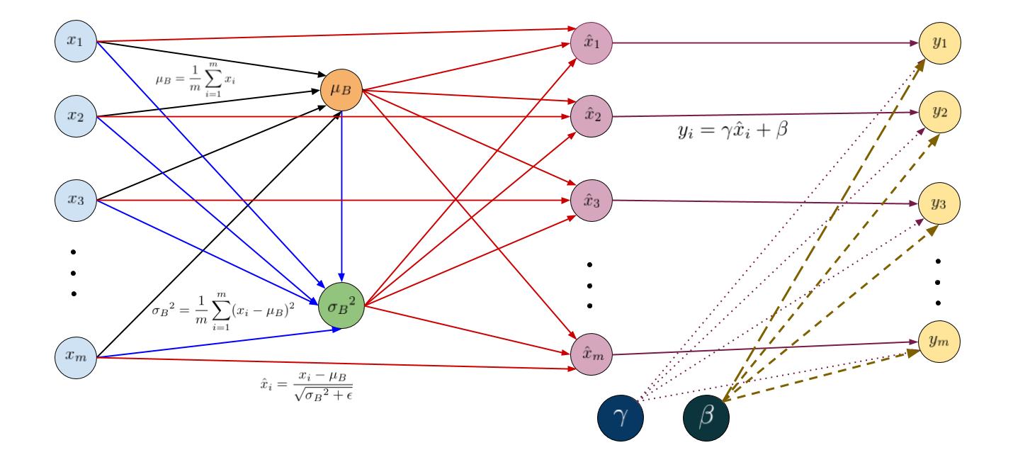
The figure given below illustrates the transformation of our inputs using a computational graph. For simplicity, we have shown the normalization of just one feature (thus dropping the superscipt \(k\)). But the idea remains the same. On left hand side are the inputs \(x_1… x_m \) to the layer (blue circles). The mean \(\mu_B\) is calculated as \(\mu_B = \frac{1}{m}\sum_{i=1}^{m}x_i \) (orange circle). Using the mean and the inputs, we compute the variance \(\sigma_B^2\) (green circle) and using inputs \(x_i\), mean \(\mu\) and variance \(\sigma_B^2\), we normalize our inputs as \(\hat{x}_i = \frac{x_i - \mu_B}{\sqrt{\sigma_B^2 + \epsilon}}\) (purple circles). The layer produces the outputs through the affine transformation \(y_i = \gamma\hat{x}_i + \beta\) (yellow circles).
Note: For in-depth discussion on computational graphs, see this blog by Christopher Olah.
Input: Values of \(x\) over a batch \(B = {x_1…x_m}\); Parameters to be learned: \(\gamma, \beta\)
Output: \({y_i = BN_{\gamma, \beta}(x_i)}\)
\[\begin{align} \mu_B &= \frac{1}{m}\sum_{i=1}^{m}x_i \\\\ \sigma_B^2 &= \frac{1}{m}\sum_{i=1}^{m}(x_i - \mu_B)^2 \\\\ \hat{x}_i &= \frac{x_i - \mu_B}{\sqrt{\sigma_B^2 + \epsilon}} \\\\ y_i &= \gamma\hat{x}_i + \beta = BN_{\gamma, \beta}(x_i) \\\\ \end{align}\]Backpropagation through Batch Normalization layer
During backpropagation, we are given the gradients of the loss with respect to the outputs (\(\frac{\partial L}{\partial y_i}\)) and are asked to calculate the gradients with respect to parameters (\(\frac{\partial L}{\partial \gamma}\) and \(\frac{\partial L}{\partial \beta}\)) and inputs (\(\frac{\partial L}{\partial x_i}\)). Using computational graph to backpropagate the error derivatives is quite simple. The only thing we have to take care of is that derivatives add up at forks. This follows the multivariable chain rule in calculus, which states that if a variable branches out to different parts of the circuit, then the gradients that flow back to it will add.
Calculation of \(\frac{\partial L}{\partial \gamma}\):
Since \(\gamma\) is used to calculate all the outputs \(y_i\) where \(i = \{1...m\}\), the gradients will be summed during backpropagation:
\[\begin{align} \frac{\partial L}{\partial \gamma} &= \sum_{i = 1}^{m}\frac{\partial L}{\partial y_i}\frac{\partial y_i}{\partial \gamma} &&&& (\text{Because gardients add up at forks})\\\\ &= \sum_{i = 1}^{m}\hat{x}_i\frac{\partial L}{\partial y_i} &&&& (\text{Because }\frac{\partial y_i}{\partial \gamma} = \hat{x}_i \text{ from } y_i = \gamma\hat{x}_i + \beta)\\\\ \end{align}\]Calculation of \(\frac{\partial L}{\partial \beta}\):
Similarly, \(\beta\) is used to calculate all the outputs \(y_i\) where \(i = \{1...m\}\), the gradients will be summed during backpropagation:
\[\begin{align} \frac{\partial L}{\partial \beta} &= \sum_{i = 1}^{m}\frac{\partial L}{\partial y_i}\frac{\partial y_i}{\partial \beta} &&&& (\text{Because gardients add up at forks})\\\\ &= \sum_{i = 1}^{m}\frac{\partial L}{\partial y_i} &&&& (\text{Because }\frac{\partial y_i}{\partial \beta} = 1 \text{ from } y_i = \gamma\hat{x}_i + \beta)\\\\ \end{align}\]Calculation of \(\frac{\partial L}{\partial \hat{x}_i}\):
\[\begin{align} \frac{\partial L}{\partial \hat{x}_i} &= \frac{\partial L}{\partial y_i}\frac{\partial y_i}{\partial \hat{x}_i} &&&&\\\\ &= \gamma\cdot\frac{\partial L}{\partial y_i} &&&&&& (\text{Because }\frac{\partial y_i}{\partial \hat{x}_i} = \gamma \text{ from } y_i = \gamma\hat{x}_i + \beta)\\\\ \end{align}\]Calculation of \(\frac{\partial L}{\partial \sigma_B^2}\):
Again, using multivariable chain rule we add the gradients coming from \(\hat{x}_i\) to compute the gradient with respect to \(\sigma_B^2\).
\[\begin{align} \frac{\partial L}{\partial \sigma_B^2} &= \sum_{i = 1}^{m}\frac{\partial L}{\partial \hat{x}_i}\frac{\partial \hat{x}_i}{\partial \sigma_B^2} &&&& (\text{Because gardients add up at forks})\\\\ &= \sum_{i = 1}^{m}\gamma\cdot\frac{\partial L}{\partial y_i}\cdot(x_i - \mu_B)\cdot\frac{-1}{2}\cdot(\sigma_B^2 + \epsilon)^{-3/2}\\\\ &\bigg(\text{Because }\frac{\partial \hat{x}_i}{\partial \sigma_B^2} = (x_i - \mu_B)\cdot\frac{-1}{2}\cdot(\sigma_B^2 + \epsilon)^{-3/2}\bigg)\\\\ &= -\gamma\cdot\frac{-1}{2}(\sigma_B^2 + \epsilon)^{(-3/2)}\sum_{i = 1}^{m}\frac{\partial L}{\partial y_i}\cdot(x_i - \mu_B) &&&& (\text{Taking out constant terms})\\\\ &= \frac{-\gamma\cdot t^3}{2}\sum_{i = 1}^{2}\frac{\partial L}{\partial y_i}\cdot(x_i - \mu_B) &&&& \boldsymbol{(\text{Let } \frac{1}{\sqrt{\sigma_B^2 + \epsilon}} = t)}\\\\ \end{align}\]Calculation of \(\frac{\partial L}{\partial \mu_B}\):
Since \(\mu_B\) is used to calculate not only \(\hat{x}_i\) but also \(\sigma_B^2\), we add the respective gradients (refer to the figure above).
\[\begin{align} \frac{\partial L}{\partial \mu_B} &= \sum_{i = 1}^{m}\frac{\partial L}{\partial \hat{x}_i}\frac{\partial \hat{x}_i}{\partial \mu_B} + \frac{\partial L}{\partial \sigma_B^2}\frac{\partial \sigma_B^2}{\partial \mu_B} &&&& (\text{Because gardients add up at forks})\\\\ &= \sum_{i = 1}^{m}\gamma\cdot\frac{\partial L}{\partial y_i}\cdot\frac{-1}{\sqrt{\sigma_B^2 + \epsilon}} + \frac{\partial L}{\partial \sigma_B^2}\cdot\frac{1}{m}\sum_{i = 1}^{m}-2(x_i-\mu_B) &&&& (\text{Because } \frac{\partial \hat{x}_i}{\partial \mu_B} = \frac{-1}{\sqrt{\sigma_B^2 + \epsilon}}\\\\ & &&&& \text{and }\frac{\partial \sigma_B^2}{\partial \mu_B} = \frac{1}{m}\sum_{i = 1}^{m}-2(x_i-\mu_B))\\\\ &= -\gamma\cdot t \sum_{i = 1}^{m}\frac{\partial L}{\partial y_i} + \frac{\partial L}{\partial \sigma_B^2}\cdot\frac{1}{m}\sum_{i = 1}^{m}-2(x_i-\mu_B)\\\\ &= -\gamma\cdot t \sum_{i = 1}^{m}\frac{\partial L}{\partial y_i} &&&& (\text{Because } \sum_{i = 1}^{m}(x_i-\mu_B) = 0)\\\\ \end{align}\]Calculation of \(\frac{\partial L}{\partial x_i}\):
If you see the computational graph, \(x_i\) is used to calculate \(\mu_B\), \(\sigma_B^2\) and \(\hat{x}_i\).
\[\begin{align} \frac{\partial L}{\partial x_i} &= \frac{\partial L}{\partial\hat{x}_i}\frac{\partial\hat{x}_i}{\partial x_i} + \frac{\partial L}{\partial\sigma_B^2}\frac{\partial\sigma_B^2}{\partial x_i} + \frac{\partial L}{\partial \mu_B}\frac{\partial\mu_B}{\partial x_i} \hspace{10 mm} (\text{Because gardients add up at forks})\\\\ &= \gamma\cdot\frac{\partial L}{\partial y_i}\cdot\frac{1}{\sqrt{\sigma_B^2 + \epsilon}} - \frac{\gamma\cdot t^3}{2}\sum_{i = 1}^{m}(\frac{\partial L}{\partial y_i}\cdot(x_i - \mu_B))\cdot\frac{2}{m}(x_i-\mu_B) - \gamma\cdot t \sum_{i = 1}^{m}(\frac{\partial L}{\partial y_i})\cdot\frac{1}{m}\\\\ & (\text{Because } \frac{\partial\hat{x}_i}{\partial x_i} = \frac{1}{\sqrt{\sigma_B^2 + \epsilon}};\hspace{10 mm} \frac{\partial\sigma_B^2}{\partial x_i} = \frac{2}{m}(x_i-\mu_B); \hspace{10 mm} \frac{\partial\mu_B}{\partial x_i} = \frac{1}{m})\\\\ &= \frac{\gamma\cdot t}{m}\bigg[m\frac{\partial L}{\partial y_i} - t^2\cdot(x_i-\mu_B)\sum_{i = 1}^{m}\frac{\partial L}{\partial y_i}(x_i - \mu_B) - \sum_{i = 1}^{m}\frac{\partial L}{\partial y_i}\bigg] \end{align}\]We have derived the expressions for the required gradients. They will be used to implement backpropagation through Batch Normalization.
Backpropagation during test time
Before we implement Batch Normalization, it is necessary to analyze its behavior during test time. Once the network has been trained, we use the normalization
\[\hat{x}^{(k)} = \frac{x^{(k)} - E[x^{(k)}]}{\sqrt{\text{Var}[x^{(k)}]}}\]using the population, rather than mini-batch statistics. Effectively, we process mini-batches of size \(m\) and use their statistics to compute:
\[\begin{align} E[x] &= E_B[\mu_B]\\\\ \text{Var}[x] &= \frac{m}{m-1}E_B[\sigma_B^2] \end{align}\]Alternatively, we can use use exponential moving average to estimate the mean and variance to be used during test time. This saves us from an extra estimation step as suggested by the paper.
During training, we estimate the running average of mean and variance as:
\[\begin{align} \mu_{running} &= \alpha\cdot\mu_{running} + (1-\alpha)\cdot\mu_B\\\\ \sigma_{running}^2 &= \alpha\cdot\sigma_{running}^2 + (1-\alpha)\cdot\sigma_{B}^2\\\\ \end{align}\]where \(\alpha\) is a constant smoothing factor between 0 and 1 and represents the degree of dependence on the previous observations. A lower \(\alpha\) discounts older observations faster. The torch implementation of Batch Normalization also uses running averages.
Python Numpy Implementation
The complete implementation of Batch Normalization can be found here. Batch Normalization layers are generally added after fully connected (or convolutional) layer and before non-linearity. In case of fully connected networks, the input X given to the layer is an \(N \times D\) matrix, where \(N\) is the batch size and \(D\) is the number of features.
batchnorm_forward API
1
2
3
4
5
6
7
8
9
10
11
12
13
14
15
16
17
18
19
20
21
22
23
24
25
26
27
28
29
30
31
32
33
34
35
36
37
38
39
40
41
42
43
44
45
46
47
48
49
50
51
52
53
54
55
def batchnorm_forward(x, gamma, beta, bn_param):
  """
  Forward pass for batch normalization.

  Input:
  - x: Data of shape (N, D)
  - gamma: Scale parameter of shape (D,)
  - beta: Shift paremeter of shape (D,)
  - bn_param: Dictionary with the following keys:
    - mode: 'train' or 'test'; required
    - eps: Constant for numeric stability
    - momentum: Constant for running mean / variance.
    - running_mean: Array of shape (D,) giving running mean of features
    - running_var Array of shape (D,) giving running variance of features

  Returns a tuple of:
  - out: of shape (N, D)
  - cache: A tuple of values needed in the backward pass
  """
  mode = bn_param['mode']
  eps = bn_param.get('eps', 1e-5)
  momentum = bn_param.get('momentum', 0.9)

  N, D = x.shape
  running_mean = bn_param.get('running_mean', np.zeros(D, dtype=x.dtype))
  running_var = bn_param.get('running_var', np.zeros(D, dtype=x.dtype))

  out, cache = None, None
  if mode == 'train':
    sample_mean = np.mean(x, axis=0)
    sample_var = np.var(x, axis=0)

    # Normalization followed by Affine transformation
    x_normalized = (x - sample_mean)/np.sqrt(sample_var + eps)
    out = gamma*x_normalized + beta

    # Estimate running average of mean and variance to use at test time
    running_mean = momentum * running_mean + (1 - momentum) * sample_mean
    running_var = momentum * running_var + (1 - momentum) * sample_var

    # Cache variables needed during backpropagation
    cache = (x, sample_mean, sample_var, gamma, beta, eps)

  elif mode == 'test':
    # normalize using running average
    x_normalized = (x - running_mean)/np.sqrt(running_var + eps)

    # Learned affine transformation
    out = gamma*x_normalized + beta

  # Store the updated running means back into bn_param
  bn_param['running_mean'] = running_mean
  bn_param['running_var'] = running_var

  return out, cache
batchnorm_backward API
1
2
3
4
5
6
7
8
9
10
11
12
13
14
15
16
17
18
19
20
21
22
23
24
25
26
27
def batchnorm_backward(dout, cache):
  """
  Backward pass for batch normalization.

  Inputs:
  - dout: Upstream derivatives, of shape (N, D)
  - cache: Variable of intermediates from batchnorm_forward.

  Returns a tuple of:
  - dx: Gradient with respect to inputs x, of shape (N, D)
  - dgamma: Gradient with respect to scale parameter gamma, of shape (D,)
  - dbeta: Gradient with respect to shift parameter beta, of shape (D,)
  """
  #Unpack cache variables
  x, sample_mean, sample_var, gamma, beta, eps = cache

  # See derivations above for dgamma, dbeta and dx
  dgamma = np.sum(dout*x_normalized, axis=0)
  dbeta = np.sum(dout, axis=0)

  m = x.shape[0]
  t = 1./np.sqrt(sample_var + eps)

  dx = (gamma * t / m) * (m * dout - np.sum(dout, axis=0)
        - t**2 * (x-sample_mean) * np.sum(dout*(x - sample_mean), axis=0))

  return dx, dgamma, dbeta
How Powerful is Batch Normalization?
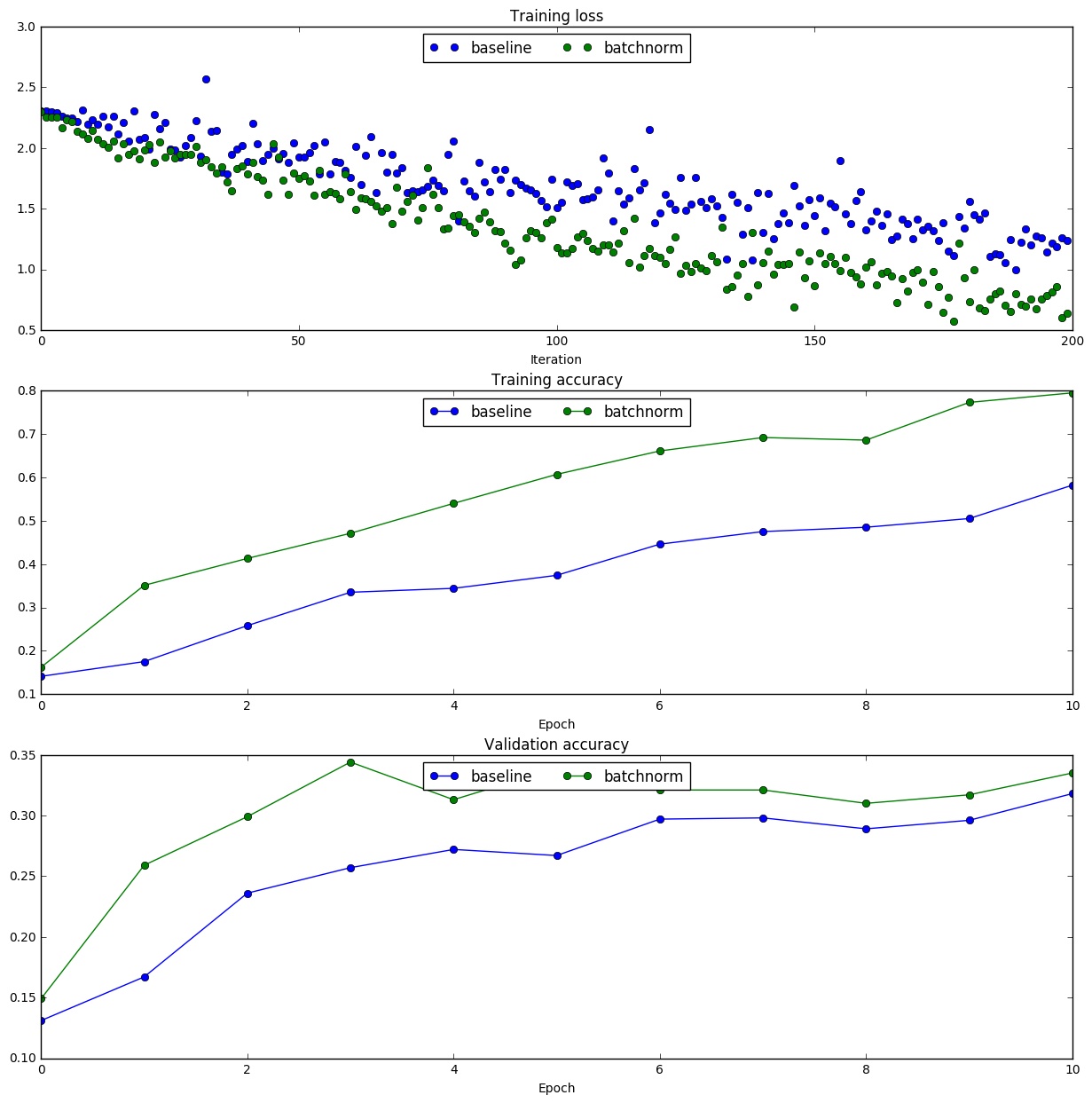
To verify our claim that Batch Normalization helps in faster convergence, we ran a small experiment with 1000 images from CIFAR-10 dataset. We plotted the training and validation accuracies against the number of epochs both with and without Batch Normalization.
To understand the effect of Batch Normalization on weight initialization, we trained 20 different networks both with and without Batch Normalization using different scales for weight initialization and plotted training accuracy, validation set accuracy and training loss.
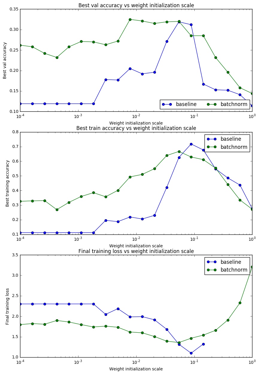
As we can see, Batch Normalization helps in faster convergence and allows less dependence on weight initialization. But there is a sweet spot at which Batch Normalization gives considerably high accuracy. Before training a neural network, proper weight scale can be estimated by running an experiment with similar setup. As the last plot suggests, without Batch Normalization the network breaks at large weight initialization scale, (may be due to lack of numerical stability), but Batch Normalization still gives some training loss.
Summary
Here are some resources that have been referred to while writing this blog.
- Batch Normalization: Accelerating Deep Network Training by Reducing Internal Covariate Shift by Sergey Ioffe and Christian Szegedy, 2015
- CS231n lecture by Andrej Karpathy
- CS231n Notes and Assignments
- Clement Thorey’s blog on Batch Normalization
Note
- Implementation of Batch Normalization using Python and Numpy was part of the assignment given by CS231n (Winter 2016). The code in this blog is taken from Yasir Mir’s GitHub repo.